Data warehouse vs Data Lake


Data Lake Vs Data warehouses

Today, my post is not technical. I would rather like to reflect on a new concept that I have been reading about Data Lakes in comparison to  Data warehouses.

Data warehouse has been around for a long time and it has proven to be effective and therefore widely used to fulfill information needs of organizations. On the other hand, Data Lake is a new phenomenon which came to existence following the boom of high data generation aka big data flood. I have read that 90% of today’s data is generated in the last 2 years. This is massive and obviously traditional data warehouses are not able to handle this. Today’s data is not just large in size. It also comes in various forms and disseminates at a very high speed. These characteristics are famously described in 3V’s (Volume – to refer to its large size, Variety – to refer to its various forms, and Velocity – to refer to the speed at which today’s data disseminates). There are other 3V’s that I came across at InsideBigdata blog as Veracity – to refer to the fact that big data is susceptible to biases and is full of noise and abnormality; Validity – meaning is the data correct and accurate for the intended use; and Volatility – refers to how long is data valid and how long should it be stored. (For more detail, see the link: http://insidebigdata.com/2013/09/12/beyond-volume-variety-velocity-issue-big-data-veracity/). Now that Data Lakes are designed in order to handle today’s large and complex data, the question is “how is it different from Data warehouse and is it intended to replace Data warehouses?”. With this in mind, I tried to investigate different views and compiled as follows.

To start with the definitions:

A data lake is defined as a storage repository that holds a vast amount of raw data in its native format until it is needed, and

A Data warehouse is defined as a subject-oriented, integrated, time-variant and non-volatile collection of data in support of the organisation’s decision making processes. The purpose of data warehouse is to integrate data from many transnational and operational systems, in order to present the resulting information as a “single integrated version of the truth” to decision makers on all levels of the organisation. The design of the data warehouse, if done properly, allows them to access, report and analyse that information from all the relevant and possible angles; in order to get consistent and accurate information as a result. Usually, different data marts to serve as the access layer of the data warehouse environment that are used to get data out to the users are built. A data mart is a subset of the data warehouse that is usually oriented to a specific business line or team. Data marts are small slices of the data warehouse.

However, there are many critiques against the data warehouse and data mart approaches. One of thse is that its careful design and subsequent implementation takes time and effort. A related critique to this is that the dimensional structures used in data warehouse and data mart are inflexible and limiting.

The proponents of Data lake argue that these problems can be avoided easily. James Dixon, the founder and CTO of Pentaho, who coined the term for the first time describes a data lake as follows.
“If you think of a data mart as a store of bottled water – cleansed and packaged and structured for easy consumption – the data lake is a large body of water in a more natural state. The contents of the data lake stream in from a source to fill the lake, and various users of the lake can come to examine, dive in, or take samples.”. Many data scientists agree today that a data lake is a storage repository that holds a vast amount of raw data in its native format, including structured, semi-structured, and unstructured data. The data structure and requirements are not defined until the data is needed. This provides flexibility for since the requirements can be defined anytime later by the business and yet the same data lake can be used to satisfy the requirement.

Due to these facts, some say “Yes” loudly to data lake and some say “No” loudly to it and in favour of data warehous. The similarity they share is simple: they both serve as storage. In order to take side, i believe it is important to understand the differences. The following table taken from kdnuggets (http://www.kdnuggets.com/) summarizes the differences.

Data warehouse vs Data Lake

Data:- A data warehouse only stores data that has been modeled/structured, while a data lake is no does not care about structure. It stores all—structured, semi-structured, and unstructured.

Processing:- Before we can load data into a data warehouse, we first need to give it some shape and structure i.e., we need to model it. That’s called schema-on-write. With a data lake, you just load in the raw data, as-is, and then when you’re ready to use the data, that’s when you give it shape and structure. That’s called schema-on-read. Two very different approaches.

Storage:- One of the primary features of big data technologies like Hadoop is that the cost of storing data is relatively low as compared to the data warehouse. There are two key reasons for this: First, Hadoop is open source software, so the licensing and community support is free. And second, Hadoop is designed to be installed on low-cost commodity hardware.

Agility:- A data warehouse is a highly-structured repository, by definition. It’s not technically hard to change the structure, but it can be very time-consuming given all the business processes that are tied to it. A data lake, on the other hand, lacks the structure of a data warehouse—which gives developers and data scientists the ability to easily configure and reconfigure their models, queries, and apps on-the-fly.

Security:- Data warehouse technologies have been around for decades, while big data technologies are relatively new. Thus, the ability to secure data in a data warehouse is much more mature than securing data in a data lake. It should be noted, however, that there’s a significant effort being placed on security right now in the big data industry. It’s not a question of if, but when.

Users:- The motto of Data Warehouse and data mart intensive environment is self-service, i.e, developing the structure and inviting users to consume information. On the other hand, data lake is not by any means easy and matured for business users to come and get useful information. It has to be still manipulated by data scientists.

As a conclusive remark, many recommend to use each according to their needs. While data warehouse is more matured, secured suitable for self service BI, data lake is suitable for storing big data characterized by the 3V’s mentioned above with low cost.

Mortgage Analytics

As a proof of concept (POC) of mortgage analytics, I did an exercise to predict borrowers turning out bad (not paying their term timely). I selected as much variables as I can and extracted from the operational database. Due to security reasons, I am not going to explain or show the data and the variables.

For demonstration purpose, I took 284 loans which are in arrear (did not pay their term) for the last 12 months (Yes) and 1049 loans which are not in arrear for the last 12 months (No). This is just a random set and as can be seen easily, the data is imbalanced as there are fewer cases where loans stay in arrear for 12 months or more.

To collect, cleanse and aggregate the data, I used T-sql since the data is stored in MSSQL server.

To analyze and visualize the data, I used R.

First, the data has to be imported as follows (the directory should be replaced with the correct path according to the user)

> datap<-read.csv(“directory/filename”)      %directory and filename should be replaced with the right values depending on the user.

Once the data is imported, different operations have to be performed to understand the data. In my case, since I used t-sql to extract the data, a lot of data cleaning is already performed.

str(datap)                         %provides the metadata info of the variables

summary(datap)            %provides the summary (min, max, median,1st,and 3rd  quartile for numeric) attributes and frequency distribution for categorical variables. Note:- if there is a big difference between mean and median, there may be an outlier.

%plotting whole dataset to have an overview of the data is difficult due to high number of variables

So subsets of data is used before plotting

eg. datasub1<-datap[,c(1:8,15)] %makes a subset of columns 1 to 8, and column 15 which is the target variable

plot(datasub1)

In addition, to understand the individual variables, a plot of each variable is done as follows:-

plot(datap$loan_income)  %to use the name of the variables directly, the dataset can be attached as follows.

Attach(datap)

scatterplot

Boxplot is much nicer in detecting outliers as can be seen as follows.

boxplot(datap$loan_income)

boxplot1

More understanding of data can also be done by different graphical forms. For example, to see the data distribution per province, a 3D pie chart can be used as follows.

pie3D(table(datap$province))

piechart1

Another important visualization could be to plot pairs of variables (one in x-axis, one on y-axis, and another as coloring etc). For example, the following is used to see the distribution of income distributed across provinces colored based on the target variable (i.e whether the loan is in arrear for the last 12 months or not).

ggplot(data = datap, aes(x= loan_income, y = province, color = Arrear12Month))+geom_point()

%ggplot2 package should be installed by using install.packages(“ggplot2”)

ggplot1


From this, Friesland tends to be clean and Flevoland tends to be sensitive (also the income distribution can be seen).  Similar graphs can be generated for other combination of variables.

Facet grids are also helpful tools to visualize data per category. Especially, it is helpful to categorize based on the target variable.

commp<-ggplot(data = datap, aes(x=commercial_prod_servicer))

> commp+geom_bar()

> commp<-commp+geom_bar()

> commp+facet_grid(.~Arrear12Month)

facet

This way, it is possible to see the influence of each variable per category.

Density plot also helps to see distributions per category as shown below.

ggplot(data = datap, aes(x= LTI, fill = Arrear12Month))+geom_density()

density

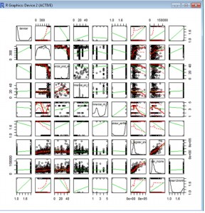
Scatter plot also gives a quick overview of relationships among variables about the data dataset. Running scatterplot on the subset of the data identified earlier as follows gives the following.

scatterplotMatrix(datasub1)   %the car package has to be installed

scatterplot2

The scatterplot shows clear relationships on some of the variables.

Another important graphical view is the corrgram depiction which shows the correlation of each variable in color matrix. Dark blue shows strong positive relationship and Dark red shows strong negative relationship. The corrgram in this dataset is given below.

library(corrgram)

corrgram(datap)   %the color coding represents (red = neg correlation, blue = positive correlation)

corrgram

After understanding the data, variables that are considered to be useful have to be selected for modelling. One can consider more advanced feature selection for a better set of variables for efficient modelling. In this case, only correlation value is used to select which features to use for modelling. So, using the selected features, the modelling is developed as follows.


%First the dataset has to be split in the form of training and test dataset (60% vs 40%)

> set.seed(2000)           %this is helpful to reproduce the random numbers again.

> d = sort(sample(nrow(datap),nrow(datap)*.6))     %sample 60% for training

> train<-datap[d, ]          %assign the 60% to training

> test<-datap[-d,]           %assign the remaining 40% for testing

%For developing the model, rpart is used as follows.

> modelsplit<-rpart(formula=Arrear12Month~Servicer+commercial_prod_servicer+commercial_ext_hds+commercial_int_hds+advisor_verified+notary_register_amount+loan_income +loan_foreclosure_value + loan_marketvalue + nhg_Ind +number_of_parts + nationality_hds +  Age + gender+ marital_state+employment_hds+gross_income+province +nr_clients + LTI + LTV +redemption_hds + application_hds , data = train, method =”class”,control=rpart.control(minsplit=10, cp=0))

> summary(modelsplit)   %dispaly the result of the model  which is stored in the modelsplit variable.

> prp(modelsplit, extra=1, uniform=F, branch=1, yesno=F, border.col=0, xsep=”/”)  %depicts graphically the result of the rpart model %libraries –rpart and rpart.plot are necessary for prp function to work

prp


%Now, we can generate the prediction for the test data and compare the test prediction result versus the actual label of the target variable

> Prediction <- predict(modelsplit, test, type = “class”)

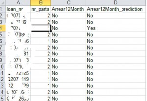
%In the following code, only the keys of the records, the target variable value, and the predicted value are chosen to make the result readable.

> submit <- data.frame(loan_nr = test$loan_nr, nr_parts = test$number_of_parts , Arrear12Month = test$Arrear12Month,Arrear12Month_prediction = Prediction)

> write.csv(submit, file = “directory”, row.names = FALSE)   %store the result in a certain directory

Now, we can check how the model performed. Some of the results are given below. In terms of accuracy, it provides 97% accuracy. Obviously, this seems to be an over fit. That is due to the amount of the dataset used (it is a very small sample to rely on).

predictionresult

In R, it is also possible to see the distribution of the data geographically. In this exercise, I took a file that contains postal codes of the Netherlands together with the corresponding latitude and longitude and I geocoded the above dataset with the help of this file (zipcode is used to link the two files).

Then I used the ggmap package  as follows:-

> install.packages(“ggmap”)  %if the package is not installed yet

> library(ggmap)

> datap2<-read.csv(“directory/filename.csv”)      %Directory and filename should be replaced with the right values depending on the user

> qmplot(lon, lat, data = datap2, colour = Arrear12Month, darken = 0.5, size =I(3.5), alpha=I(.6), legend = ‘topleft’) %depicts the dataset on the map.

ggmap


SAP Business Objects 4.x Backup and Restore

We all know that since SAP upgraded BO to 4.x, the backup and restore process has been a difficult job. BO admins know what I am talking about. The import/export wizard that was available in version 3.0 is gone, rather a web-based LCM tool is integrated. The problem with this is that it is not dependable for backing up and restoring large files. There are two possibilities to create a backup: using the web interface tool and using a command line tool. The funny thing is, if the back up is taken using the web interface, it can only be restored using the web interface again and still requires the backup job to be available. The same story for command line.

In our company, we split the backup in to 3 different jobs.

  1. Universes, connections, users, groups and profiles using the web interface tool.
  2. Personal folders using web interface.
  3. All the folders (this is huge in size) using the command line.

We tested the procedures to back up and restore using small size of files and that worked fine and we never tried to recover the whole file.

Recently, a guy has deleted a very important folder in their department by mistake and everybody started panicking. He immediately called for help. Now comes the real challenge :). Oh, did I also mention that selective restore is not possible in BO 4? It is unthinkable that you can only restore the whole backup. We cannot do that on production system because the other users will be affected. Fortunately, I kind of foresee the problem and have asked a sandbox server. It was a hassle to get the server (took about 6 months) and my manager interfered and we got it. So, i installed BO on the sandbox server and we use it to test new patches and service packs. So, for this problem to recover our lost folder, I tried to restore back up #3 (see above) to the sandbox server hoping that I will use promotion management to take the folder to production after restore. However, when the restore is finished, the folder I want is not there. Apparently, it seems the back up is not complete. In the mean time, these people who use the folder are calling and asking me the status. This is getting serious. We cannot afford loosing this folder. It contains important reports and people (including myself) have worked hard to get those reports in place. So,time to think!

Finally, I decided to go for a complete restore. I followed the following steps.

  1. I took the Filestore backup of the production system and copied it to the Sandbox system with a different name.
  2. I took the CMS dabase backup of the production system and restored it to the sandbox system with a different name.
  3. I stopped tomcat and SIA on the sandbox.
  4. I renamed the existing Filestore to a different name and renamed the file of #1 to Filestore.
  5. Then I created a new node (SIA), this is important, and pointed it to the new database restored. A lot of attention is needed here. The SIA has to be created with default servers and the access key used when the production system was configured has to be supplied.
  6. Then started tomcat and SIA.
  7. When everything started, I logged to CMC of the sandbox systems and checked everything. It looked fine. I created a job and promoted the folder needed to production and the reports run as normal. Everybody was happy and it was a nice excercise for me as well.